18 Exercise 2: Dictionary-based methods
18.1 Introduction
In this tutorial, you will learn how to:
- Use dictionary-based techniques to analyze text
- Use common sentiment dictionaries
- Create your own “dictionary”
- Use the Lexicoder sentiment dictionary from Young and Soroka (2012)
18.2 Setup
The hands-on exercise for this week uses dictionary-based methods for filtering and scoring words. Dictionary-based methods use pre-generated lexicons, which are no more than list of words with associated scores or variables measuring the valence of a particular word. In this sense, the exercise is not unlike our analysis of Edinburgh Book Festival event descriptions. Here, we were filtering descriptions based on the presence or absence of a word related to women or gender. We can understand this approach as a particularly simple type of “dictionary-based” method. Here, our “dictionary” or “lexicon” contained just a few words related to gender.
18.3 Load data and packages
Before proceeding, we’ll load the remaining packages we will need for this tutorial.
library(academictwitteR) # for fetching Twitter data
library(tidyverse) # loads dplyr, ggplot2, and others
library(readr) # more informative and easy way to import data
library(stringr) # to handle text elements
library(tidytext) # includes set of functions useful for manipulating text
library(quanteda) # includes functions to implement Lexicoder
library(textdata)
In this exercise we’ll be using another new dataset. The data were collected from the Twitter accounts of the top eight newspapers in the UK by circulation. You can see the names of the newspapers in the code below:
newspapers = c("TheSun", "DailyMailUK", "MetroUK", "DailyMirror",
               "EveningStandard", "thetimes", "Telegraph", "guardian")

tweets <-
  get_all_tweets(
    users = newspapers,
    start_tweets = "2020-01-01T00:00:00Z",
    end_tweets = "2020-05-01T00:00:00Z",
    data_path = "data/sentanalysis/",
    n = Inf,
  )

tweets <-
  bind_tweets(data_path = "data/sentanalysis/", output_format = "tidy")

saveRDS(tweets, "data/sentanalysis/newstweets.rds")
For details of how to access Twitter data with academictwitteR, check out details of the package here.
We can download the final dataset with:
tweets <- readRDS("data/sentanalysis/newstweets.rds")If you’re working on this document from your own computer (“locally”) you can download the tweets data in the following way:
18.4 Inspect and filter data
Let’s have a look at the data:
head(tweets)## # A tibble: 6 × 31
## tweet_id user_username text lang author_id source
## <chr> <chr> <chr> <chr> <chr> <chr>
## 1 1212334402266521602 DailyMirror "Secr… en 16887175 Tweet…
## 2 1212334169457676289 DailyMirror "RT @… en 16887175 Tweet…
## 3 1212333195879993344 thetimes "A ce… en 6107422 Echob…
## 4 1212333194864988161 TheSun "Wayn… en 34655603 Echob…
## 5 1212332920507191296 DailyMailUK "Stud… en 111556423 Socia…
## 6 1212332640570875904 TheSun "Dad … en 34655603 Twitt…
## # ℹ 25 more variables: possibly_sensitive <lgl>,
## # conversation_id <chr>, created_at <chr>, user_url <chr>,
## # user_location <chr>, user_protected <lgl>,
## # user_verified <lgl>, user_name <chr>,
## # user_profile_image_url <chr>, user_description <chr>,
## # user_created_at <chr>, user_pinned_tweet_id <chr>,
## # retweet_count <int>, like_count <int>, quote_count <int>, …
colnames(tweets)## [1] "tweet_id" "user_username"
## [3] "text" "lang"
## [5] "author_id" "source"
## [7] "possibly_sensitive" "conversation_id"
## [9] "created_at" "user_url"
## [11] "user_location" "user_protected"
## [13] "user_verified" "user_name"
## [15] "user_profile_image_url" "user_description"
## [17] "user_created_at" "user_pinned_tweet_id"
## [19] "retweet_count" "like_count"
## [21] "quote_count" "user_tweet_count"
## [23] "user_list_count" "user_followers_count"
## [25] "user_following_count" "sourcetweet_type"
## [27] "sourcetweet_id" "sourcetweet_text"
## [29] "sourcetweet_lang" "sourcetweet_author_id"
## [31] "in_reply_to_user_id"Each row here is a tweets produced by one of the news outlets detailed above over a five month period, January–May 2020. Note also that each tweets has a particular date. We can therefore use these to look at any over time changes.
We won’t need all of these variables so let’s just keep those that are of interest to us:
tweets <- tweets %>%
  select(user_username, text, created_at, user_name,
         retweet_count, like_count, quote_count) %>%
  rename(username = user_username,
         newspaper = user_name,
tweet = text)| username | tweet | created_at | newspaper | retweet_count | like_count | quote_count |
|---|---|---|---|---|---|---|
| EveningStandard | We can’t complain: Two men spend coronavirus lockdown in London pub with ‘fresh beer on tap’ 🍺 https://t.co/rG65nGWv6q | 2020-04-30T23:43:24.000Z | Evening Standard | 3 | 4 | 0 |
| EveningStandard | Best home spa treatments: face, body, nail and hair products for home https://t.co/nDZ65BbbVs | 2020-04-30T23:57:09.000Z | Evening Standard | 0 | 2 | 0 |
| guardian | Coronavirus live news: Trump claims to have evidence virus started in Wuhan lab as UK is ‘past the peak’ https://t.co/LZv4yx2kn2 | 2020-04-30T23:57:59.000Z | The Guardian | 19 | 40 | 8 |
| guardian | Rugby league gets £16m emergency loan from government https://t.co/kZ9PP4aWjO | 2020-04-30T23:57:59.000Z | The Guardian | 9 | 12 | 0 |
| guardian | Coronavirus latest: at a glance https://t.co/OrWrEdOwoU | 2020-04-30T23:58:01.000Z | The Guardian | 8 | 11 | 3 |
We manipulate the data into tidy format again, unnesting each token (here: words) from the tweet text.
tidy_tweets <- tweets %>%
  mutate(desc = tolower(tweet)) %>%
  unnest_tokens(word, desc) %>%
  filter(str_detect(word, "[a-z]"))
We’ll then tidy this further, as in the previous example, by removing stop words:
18.5 Get sentiment dictionaries
Several sentiment dictionaries come bundled with the tidytext package. These are:
-
AFINNfrom Finn Årup Nielsen, -
bingfrom Bing Liu and collaborators, and -
nrcfrom Saif Mohammad and Peter Turney
We can have a look at some of these to see how the relevant dictionaries are stored.
get_sentiments("afinn")## # A tibble: 2,477 × 2
## word value
## <chr> <dbl>
## 1 abandon -2
## 2 abandoned -2
## 3 abandons -2
## 4 abducted -2
## 5 abduction -2
## 6 abductions -2
## 7 abhor -3
## 8 abhorred -3
## 9 abhorrent -3
## 10 abhors -3
## # ℹ 2,467 more rows
get_sentiments("bing")## # A tibble: 6,786 × 2
## word sentiment
## <chr> <chr>
## 1 2-faces negative
## 2 abnormal negative
## 3 abolish negative
## 4 abominable negative
## 5 abominably negative
## 6 abominate negative
## 7 abomination negative
## 8 abort negative
## 9 aborted negative
## 10 aborts negative
## # ℹ 6,776 more rows
get_sentiments("nrc")## # A tibble: 13,875 × 2
## word sentiment
## <chr> <chr>
## 1 abacus trust
## 2 abandon fear
## 3 abandon negative
## 4 abandon sadness
## 5 abandoned anger
## 6 abandoned fear
## 7 abandoned negative
## 8 abandoned sadness
## 9 abandonment anger
## 10 abandonment fear
## # ℹ 13,865 more rowsWhat do we see here. First, the AFINN lexicon gives words a score from -5 to +5, where more negative scores indicate more negative sentiment and more positive scores indicate more positive sentiment. The nrc lexicon opts for a binary classification: positive, negative, anger, anticipation, disgust, fear, joy, sadness, surprise, and trust, with each word given a score of 1/0 for each of these sentiments. In other words, for the nrc lexicon, words appear multiple times if they enclose more than one such emotion (see, e.g., “abandon” above). The bing lexicon is most minimal, classifying words simply into binary “positive” or “negative” categories.
Let’s see how we might filter the texts by selecting a dictionary, or subset of a dictionary, and using inner_join() to then filter out tweet data. We might, for example, be interested in fear words. Maybe, we might hypothesize, there is a uptick of fear toward the beginning of the coronavirus outbreak. First, let’s have a look at the words in our tweet data that the nrc lexicon codes as fear-related words.
nrc_fear <- get_sentiments("nrc") %>%
  filter(sentiment == "fear")

tidy_tweets %>%
  inner_join(nrc_fear) %>%
  count(word, sort = TRUE)
## Joining with `by = join_by(word)`## # A tibble: 1,173 × 2
## word n
## <chr> <int>
## 1 mum 4509
## 2 death 4073
## 3 police 3275
## 4 hospital 2240
## 5 government 2179
## 6 pandemic 1877
## 7 fight 1309
## 8 die 1199
## 9 attack 1099
## 10 murder 1064
## # ℹ 1,163 more rowsWe have a total of 1,174 words with some fear valence in our tweet data according to the nrc classification. Several seem reasonable (e.g., “death,” “pandemic”); others seems less so (e.g., “mum,” “fight”).
18.6 Sentiment trends over time
Do we see any time trends? First let’s make sure the data are properly arranged in ascending order by date. We’ll then add column, which we’ll call “order,” the use of which will become clear when we do the sentiment analysis.
#gen data variable, order and format date
tidy_tweets$date <- as.Date(tidy_tweets$created_at)

tidy_tweets <- tidy_tweets %>%
  arrange(date)

tidy_tweets$order <- 1:nrow(tidy_tweets)
Remember that the structure of our tweet data is in a one token (word) per document (tweet) format. In order to look at sentiment trends over time, we’ll need to decide over how many words to estimate the sentiment.
In the below, we first add in our sentiment dictionary with inner_join(). We then use the count() function, specifying that we want to count over dates, and that words should be indexed in order (i.e., by row number) over every 1000 rows (i.e., every 1000 words).
This means that if one date has many tweets totalling >1000 words, then we will have multiple observations for that given date; if there are only one or two tweets then we might have just one row and associated sentiment score for that date.
We then calculate the sentiment scores for each of our sentiment types (positive, negative, anger, anticipation, disgust, fear, joy, sadness, surprise, and trust) and use the spread() function to convert these into separate columns (rather than rows). Finally we calculate a net sentiment score by subtracting the score for negative sentiment from positive sentiment.
#get tweet sentiment by date
tweets_nrc_sentiment <- tidy_tweets %>%
  inner_join(get_sentiments("nrc")) %>%
  count(date, index = order %/% 1000, sentiment) %>%
  spread(sentiment, n, fill = 0) %>%
  mutate(sentiment = positive - negative)
## Joining with `by = join_by(word)`## Warning in inner_join(., get_sentiments("nrc")): Detected an unexpected many-to-many relationship between `x` and
## `y`.
## ℹ Row 2 of `x` matches multiple rows in `y`.
## ℹ Row 7712 of `y` matches multiple rows in `x`.
## ℹ If a many-to-many relationship is expected, set `relationship
## = "many-to-many"` to silence this warning.
tweets_nrc_sentiment %>%
  ggplot(aes(date, sentiment)) +
  geom_point(alpha=0.5) +
  geom_smooth(method= loess, alpha=0.25)
## `geom_smooth()` using formula = 'y ~ x'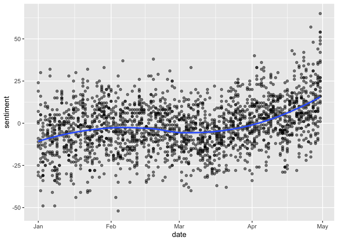
How do our different sentiment dictionaries look when compared to each other? We can then plot the sentiment scores over time for each of our sentiment dictionaries like so:
tidy_tweets %>%
  inner_join(get_sentiments("bing")) %>%
  count(date, index = order %/% 1000, sentiment) %>%
  spread(sentiment, n, fill = 0) %>%
  mutate(sentiment = positive - negative) %>%
  ggplot(aes(date, sentiment)) +
  geom_point(alpha=0.5) +
  geom_smooth(method= loess, alpha=0.25) +
  ylab("bing sentiment")
## Joining with `by = join_by(word)`## Warning in inner_join(., get_sentiments("bing")): Detected an unexpected many-to-many relationship between `x` and
## `y`.
## ℹ Row 54114 of `x` matches multiple rows in `y`.
## ℹ Row 3848 of `y` matches multiple rows in `x`.
## ℹ If a many-to-many relationship is expected, set `relationship
## = "many-to-many"` to silence this warning.## `geom_smooth()` using formula = 'y ~ x'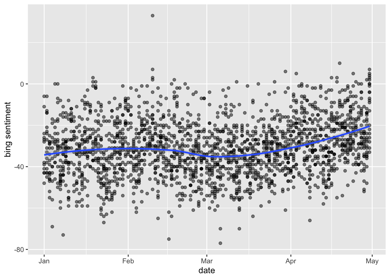
tidy_tweets %>%
  inner_join(get_sentiments("nrc")) %>%
  count(date, index = order %/% 1000, sentiment) %>%
  spread(sentiment, n, fill = 0) %>%
  mutate(sentiment = positive - negative) %>%
  ggplot(aes(date, sentiment)) +
  geom_point(alpha=0.5) +
  geom_smooth(method= loess, alpha=0.25) +
  ylab("nrc sentiment")
## Joining with `by = join_by(word)`## Warning in inner_join(., get_sentiments("nrc")): Detected an unexpected many-to-many relationship between `x` and
## `y`.
## ℹ Row 2 of `x` matches multiple rows in `y`.
## ℹ Row 7712 of `y` matches multiple rows in `x`.
## ℹ If a many-to-many relationship is expected, set `relationship
## = "many-to-many"` to silence this warning.## `geom_smooth()` using formula = 'y ~ x'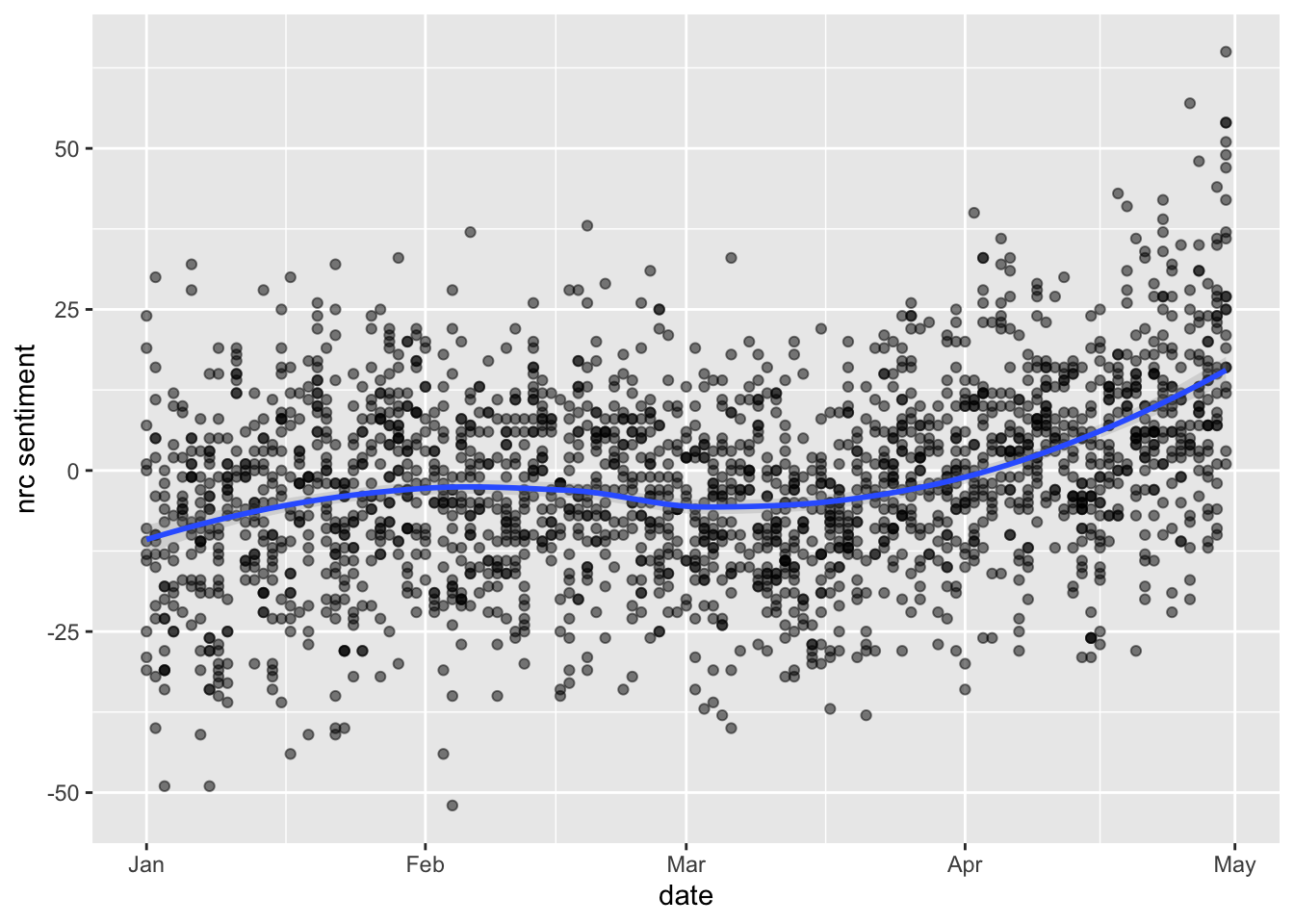
tidy_tweets %>%
  inner_join(get_sentiments("afinn")) %>%
  group_by(date, index = order %/% 1000) %>%
  summarise(sentiment = sum(value)) %>%
  ggplot(aes(date, sentiment)) +
  geom_point(alpha=0.5) +
  geom_smooth(method= loess, alpha=0.25) +
  ylab("afinn sentiment")
## Joining with `by = join_by(word)`
## `summarise()` has grouped output by 'date'. You can override
## using the `.groups` argument.
## `geom_smooth()` using formula = 'y ~ x'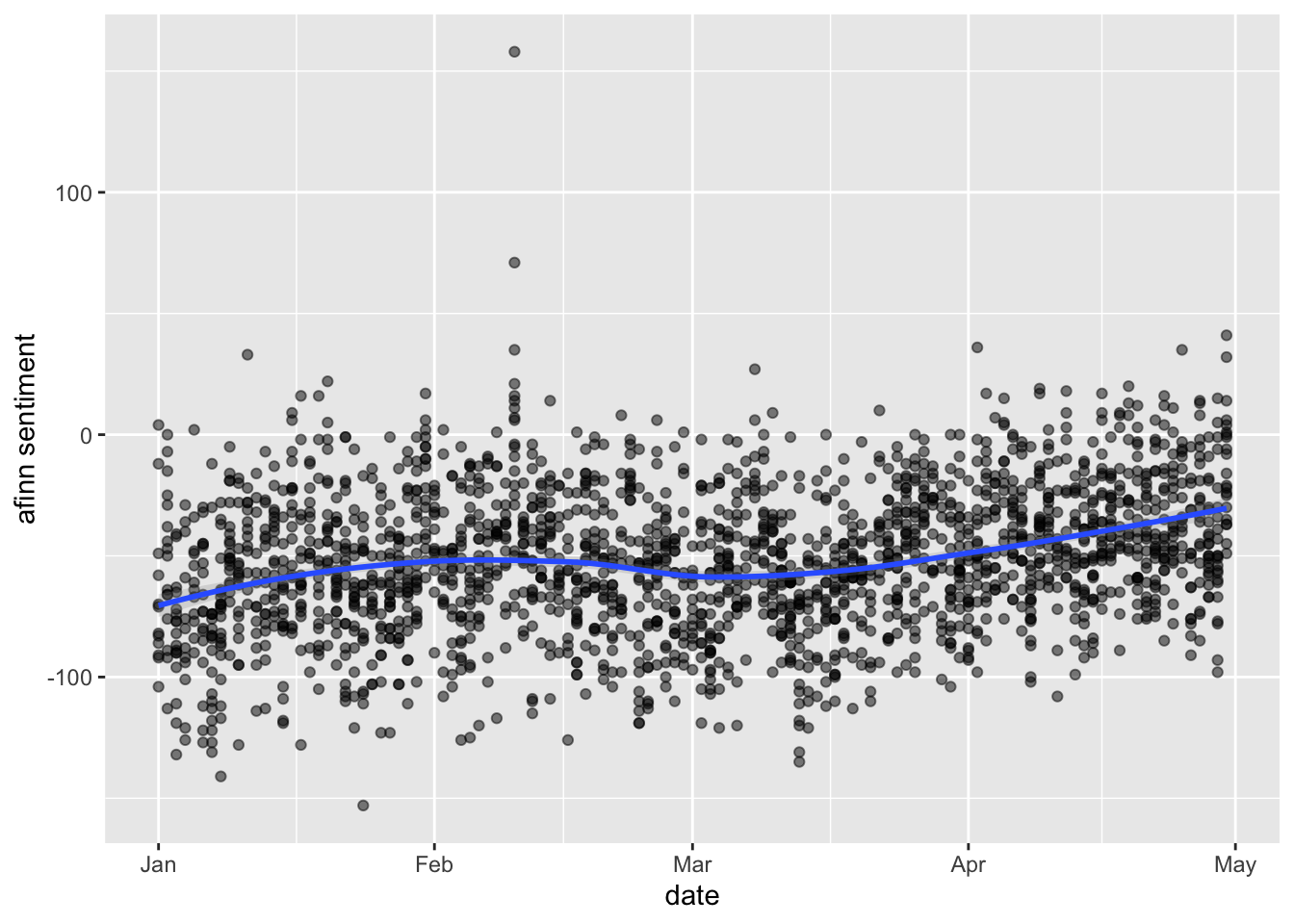
We see that they do look pretty similar… and interestingly it seems that overall sentiment positivity increases as the pandemic breaks.
18.7 Domain-specific lexicons
Of course, list- or dictionary-based methods need not only focus on sentiment, even if this is one of their most common uses. In essence, what you’ll have seen from the above is that sentiment analysis techniques rely on a given lexicon and score words appropriately. And there is nothing stopping us from making our own dictionaries, whether they measure sentiment or not. In the data above, we might be interested, for example, in the prevalence of mortality-related words in the news. As such, we might choose to make our own dictionary of terms. What would this look like?
A very minimal example would choose, for example, words like “death” and its synonyms and score these all as 1. We would then combine these into a dictionary, which we’ve called “mordict” here.
word <- c('death', 'illness', 'hospital', 'life', 'health',
             'fatality', 'morbidity', 'deadly', 'dead', 'victim')
value <- c(1, 1, 1, 1, 1, 1, 1, 1, 1, 1)
mordict <- data.frame(word, value)
mordict
## word value
## 1 death 1
## 2 illness 1
## 3 hospital 1
## 4 life 1
## 5 health 1
## 6 fatality 1
## 7 morbidity 1
## 8 deadly 1
## 9 dead 1
## 10 victim 1We could then use the same technique as above to bind these with our data and look at the incidence of such words over time. Combining the sequence of scripts from above we would do the following:
tidy_tweets %>%
  inner_join(mordict) %>%
  group_by(date, index = order %/% 1000) %>%
  summarise(morwords = sum(value)) %>%
  ggplot(aes(date, morwords)) +
  geom_bar(stat= "identity") +
  ylab("mortality words")
## Joining with `by = join_by(word)`
## `summarise()` has grouped output by 'date'. You can override
## using the `.groups` argument.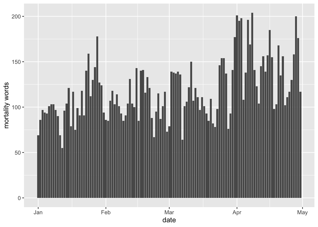
The above simply counts the number of mortality words over time. This might be misleading if there are, for example, more or longer tweets at certain points in time; i.e., if the length or quantity of text is not time-constant.
Why would this matter? Well, in the above it could just be that we have more mortality words later on because there are just more tweets earlier on. By just counting words, we are not taking into account the denominator.
An alternative, and preferable, method here would simply take a character string of the relevant words. We would then sum the total number of words across all tweets over time. Then we would filter our tweet words by whether or not they are a mortality word or not, according to the dictionary of words we have constructed. We would then do the same again with these words, summing the number of times they appear for each date.
After this, we join with our data frame of total words for each date. Note that here we are using full_join() as we want to include dates that appear in the “totals” data frame that do not appear when we filter for mortality words; i.e., days when mortality words are equal to 0. We then go about plotting as before.
mordict <- c('death', 'illness', 'hospital', 'life', 'health',
             'fatality', 'morbidity', 'deadly', 'dead', 'victim')

#get total tweets per day (no missing dates so no date completion required)
totals <- tidy_tweets %>%
  mutate(obs=1) %>%
  group_by(date) %>%
  summarise(sum_words = sum(obs))

#plot
tidy_tweets %>%
  mutate(obs=1) %>%
  filter(grepl(paste0(mordict, collapse = "|"),word, ignore.case = T)) %>%
  group_by(date) %>%
  summarise(sum_mwords = sum(obs)) %>%
  full_join(totals, word, by="date") %>%
  mutate(sum_mwords= ifelse(is.na(sum_mwords), 0, sum_mwords),
         pctmwords = sum_mwords/sum_words) %>%
  ggplot(aes(date, pctmwords)) +
  geom_point(alpha=0.5) +
  geom_smooth(method= loess, alpha=0.25) +
  xlab("Date") + ylab("% mortality words")
## `geom_smooth()` using formula = 'y ~ x'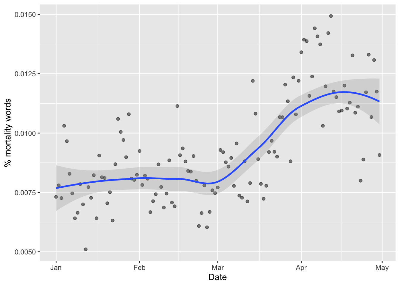
18.8 Using Lexicoder
The above approaches use general dictionary-based techniques that were not designed for domain-specific text such as news text. The Lexicoder Sentiment Dictionary, by Young and Soroka (2012) was designed specifically for examining the affective content of news text. In what follows, we will see how to implement an analysis using this dictionary.
We will conduct the analysis using the quanteda package. You will see that we can tokenize text in a similar way using functions included in the quanteda package.
With the quanteda package we first need to create a “corpus” object, by declaring our tweets a corpus object. Here, we make sure our date column is correctly stored and then create the corpus object with the corpus() function. Note that we are specifying the text_field as “tweet” as this is where our text data of interest is, and we are including information on the date that tweet was published. This information is specified with the docvars argument. You’ll see tthen that the corpus consists of the text and so-called “docvars,” which are just the variables (columns) in the original dataset. Here, we have only included the date column.
tweets$date <- as.Date(tweets$created_at)

tweet_corpus <- corpus(tweets, text_field = "tweet", docvars = "date")
## Warning: docvars argument is not used.We then tokenize our text using the tokens() function from quanteda, removing punctuation along the way:
toks_news <- tokens(tweet_corpus, remove_punct = TRUE)We then take the data_dictionary_LSD2015 that comes bundled with quanteda and and we select only the positive and negative categories, excluding words deemed “neutral.” After this, we are ready to “look up” in this dictionary how the tokens in our corpus are scored with the tokens_lookup() function.
# select only the "negative" and "positive" categories
data_dictionary_LSD2015_pos_neg <- data_dictionary_LSD2015[1:2]

toks_news_lsd <- tokens_lookup(toks_news, dictionary = data_dictionary_LSD2015_pos_neg)
This creates a long list of all the texts (tweets) annotated with a series of ‘positive’ or ‘negative’ annotations depending on the valence of the words in that text. The creators of quanteda then recommend we generate a document feature matric from this. Grouping by date, we then get a dfm object, which is a quite convoluted list object that we can plot using base graphics functions for plotting matrices.
# create a document document-feature matrix and group it by date
dfmat_news_lsd <- dfm(toks_news_lsd) %>%
  dfm_group(groups = date)

# plot positive and negative valence over time
matplot(dfmat_news_lsd$date, dfmat_news_lsd, type = "l", lty = 1, col = 1:2,
        ylab = "Frequency", xlab = "")
grid()
legend("topleft", col = 1:2, legend = colnames(dfmat_news_lsd), lty = 1, bg = "white")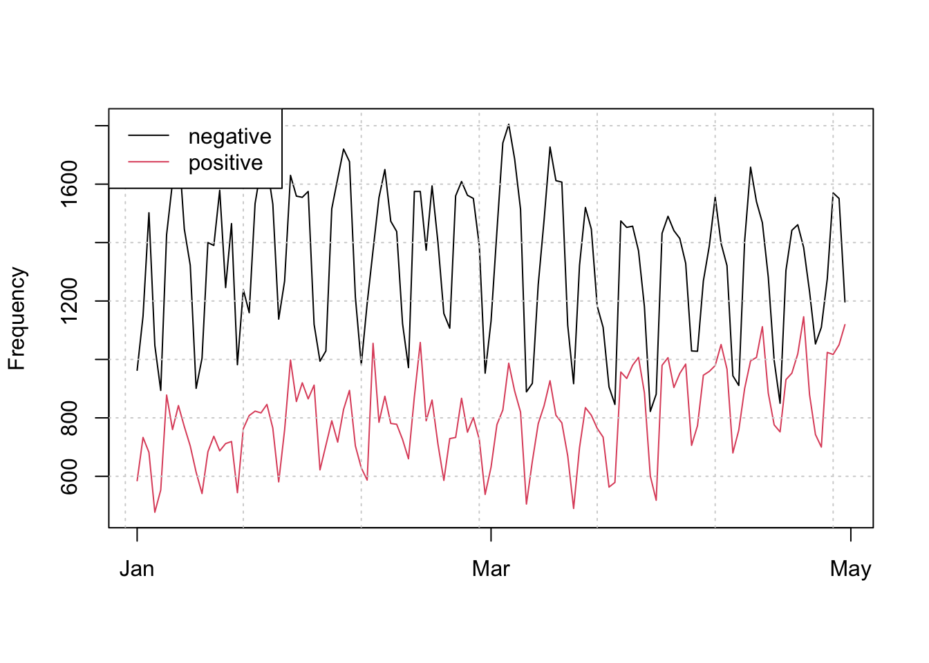
# plot overall sentiment (positive  - negative) over time

plot(dfmat_news_lsd$date, dfmat_news_lsd[,"positive"] - dfmat_news_lsd[,"negative"],
     type = "l", ylab = "Sentiment", xlab = "")
grid()
abline(h = 0, lty = 2)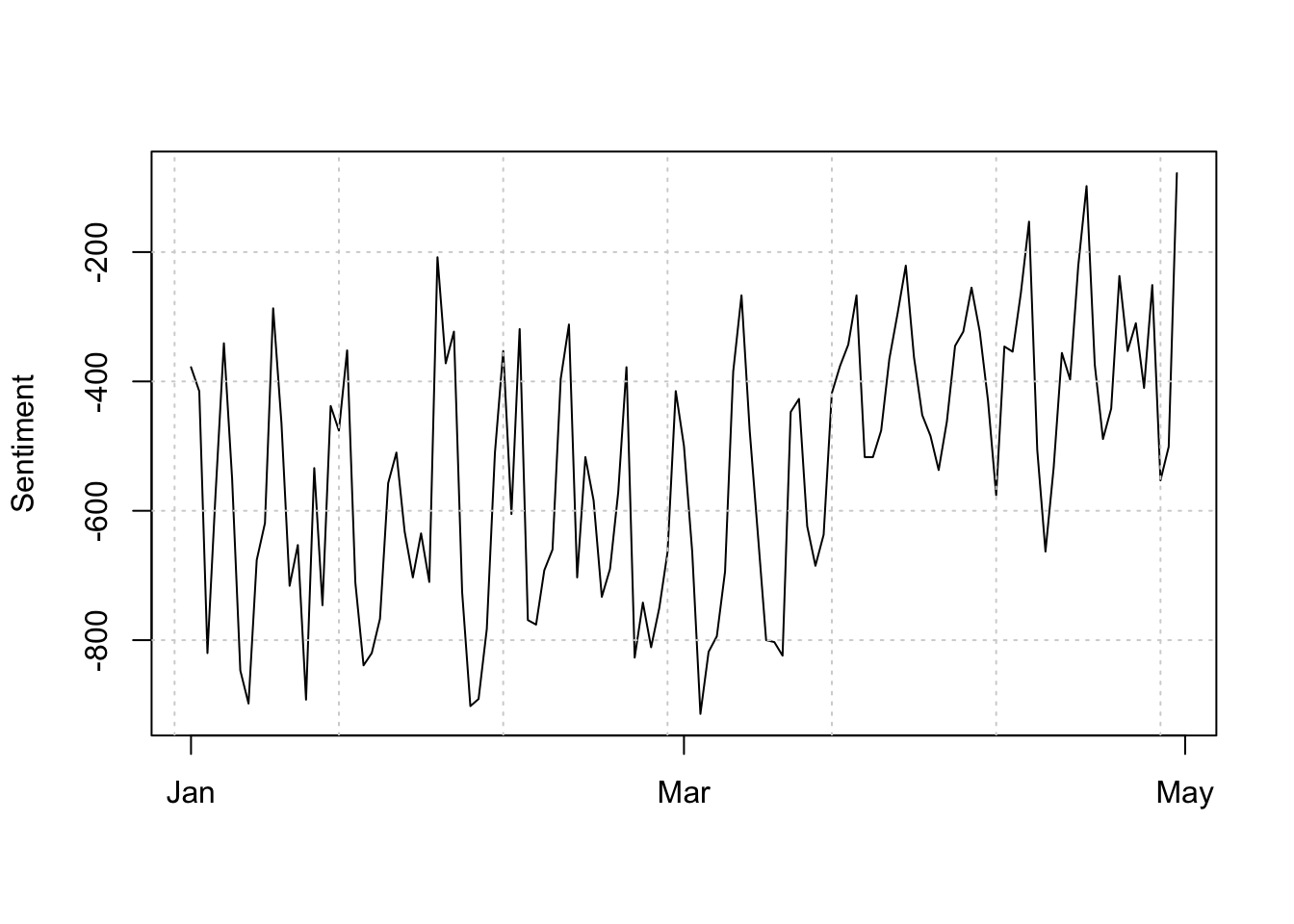
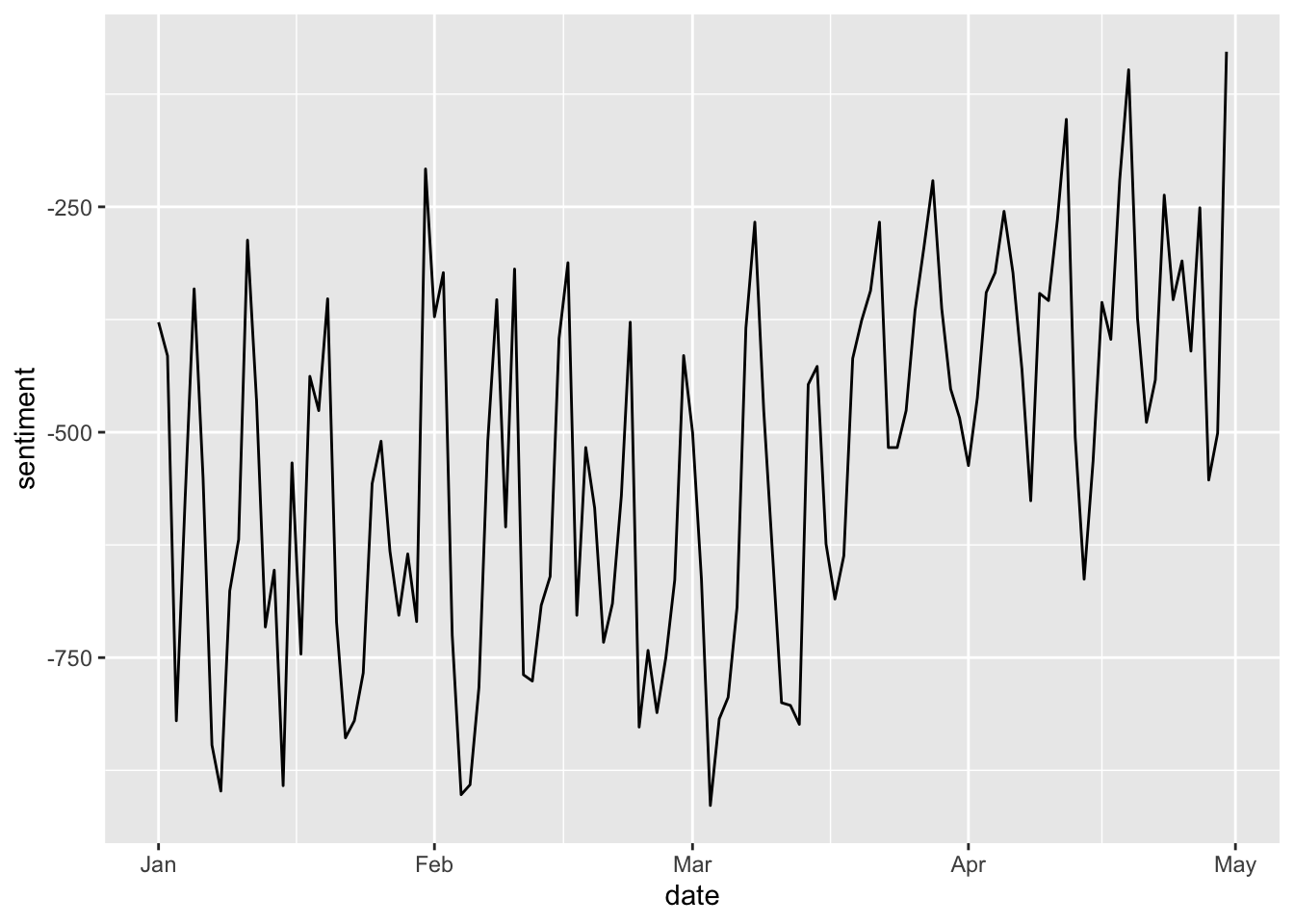
Alternatively, we can recreate this in tidy format as follows:
negative <- dfmat_news_lsd@x[1:121]
positive <- dfmat_news_lsd@x[122:242]
date <- dfmat_news_lsd@Dimnames$docs


tidy_sent <- as.data.frame(cbind(negative, positive, date))

tidy_sent$negative <- as.numeric(tidy_sent$negative)
tidy_sent$positive <- as.numeric(tidy_sent$positive)
tidy_sent$sentiment <- tidy_sent$positive - tidy_sent$negative
tidy_sent$date <- as.Date(tidy_sent$date)
And plot accordingly:
18.9 Exercises
- Take a subset of the tweets data by “user_name” These names describe the name of the newspaper source of the Twitter account. Do we see different sentiment dynamics if we look only at different newspaper sources?
- Build your own (minimal) dictionary-based filter technique and plot the result
- Apply the Lexicoder Sentiment Dictionary to the news tweets, but break down the analysis by newspaper