5 Week 3 Demo
In this section, we’ll have a quick overview of how we’re processing text data when conducting basic sentiment analyses.
5.2 Happy words
As we discussed in the lectures, we might find in our text of the class’s collective thoughts that there was an increase in “happy” words over time.
I have simulated a dataset of text split by weeks, students, and words plus whether or not the word is the word “happy” where 0 means it is not the word “happy” and 1 means it is.
We have three datasets: one with a constant number of “happy” words; one with an increasing number of “happy” words; and one with a decreasing number of “happy” words. These are called: happyn, happyu, and happyd respectively.
head(happyn)## # A tibble: 6 × 4
## # Groups: week, student [1]
## week student word happy
## <int> <int> <chr> <int>
## 1 1 9 lorem 0
## 2 1 9 ipsum 0
## 3 1 9 dolor 0
## 4 1 9 sit 0
## 5 1 9 amet 0
## 6 1 9 nam 0
head(happyu)## # A tibble: 6 × 4
## # Groups: week, student [1]
## week student word happy
## <int> <int> <chr> <int>
## 1 1 9 lorem 0
## 2 1 9 ipsum 0
## 3 1 9 dolor 0
## 4 1 9 sit 0
## 5 1 9 amet 0
## 6 1 9 nam 0
head(happyd)## # A tibble: 6 × 4
## # Groups: week, student [1]
## week student word happy
## <int> <int> <chr> <int>
## 1 1 9 lorem 0
## 2 1 9 ipsum 0
## 3 1 9 dolor 0
## 4 1 9 sit 0
## 5 1 9 amet 0
## 6 1 9 nam 0We can then see the trend in “happy” words over by week and student.
First, the dataset where we have a constant number of happy words over time.
## Warning: Returning more (or less) than 1 row per `summarise()` group was
## deprecated in dplyr 1.1.0.
## ℹ Please use `reframe()` instead.
## ℹ When switching from `summarise()` to `reframe()`, remember
##   that `reframe()` always returns an ungrouped data frame and
##   adjust accordingly.
## Call `lifecycle::last_lifecycle_warnings()` to see where this
## warning was generated.
## `summarise()` has grouped output by 'week', 'student'. You can
## override using the `.groups` argument.
## `geom_smooth()` using method = 'loess' and formula = 'y ~ x'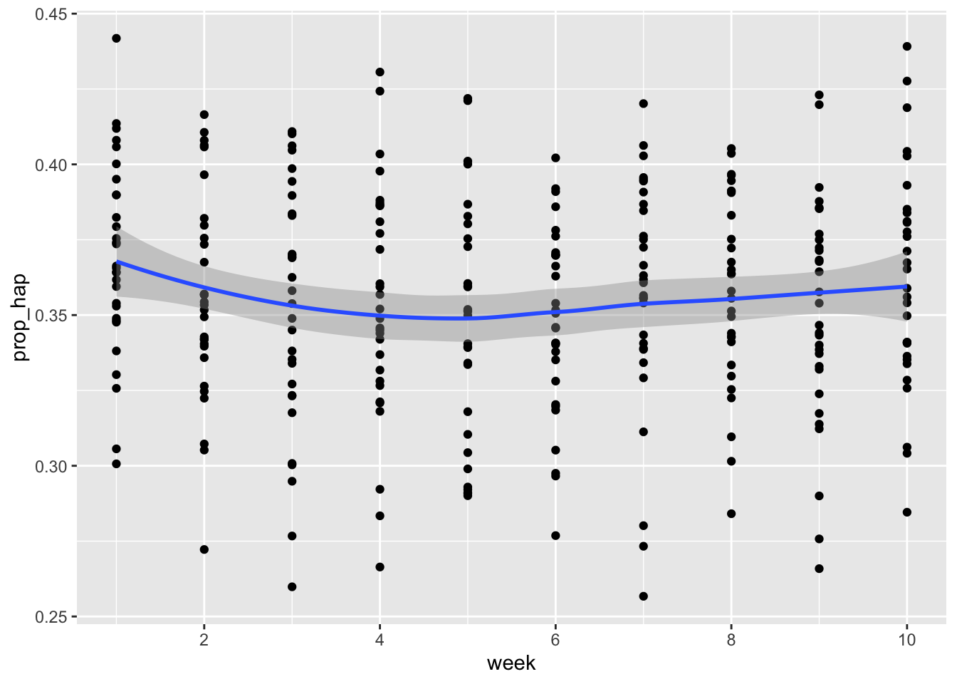
And now the simulated data with an increasing number of happy words.
## Warning: Returning more (or less) than 1 row per `summarise()` group was
## deprecated in dplyr 1.1.0.
## ℹ Please use `reframe()` instead.
## ℹ When switching from `summarise()` to `reframe()`, remember
##   that `reframe()` always returns an ungrouped data frame and
##   adjust accordingly.
## Call `lifecycle::last_lifecycle_warnings()` to see where this
## warning was generated.
## `summarise()` has grouped output by 'week', 'student'. You can
## override using the `.groups` argument.
## `geom_smooth()` using method = 'loess' and formula = 'y ~ x'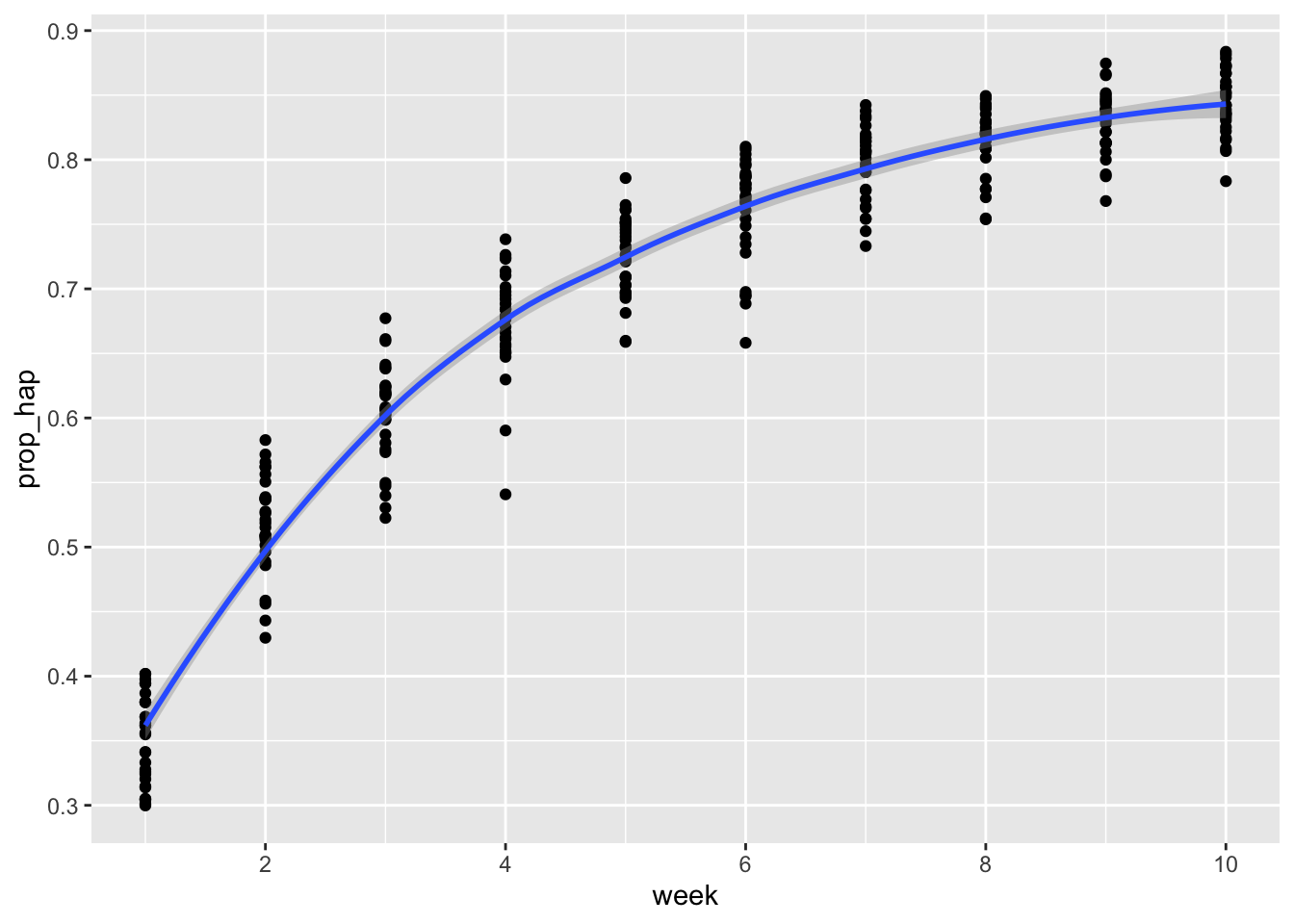
And finally a decreasing number of happy words.
## Warning: Returning more (or less) than 1 row per `summarise()` group was
## deprecated in dplyr 1.1.0.
## ℹ Please use `reframe()` instead.
## ℹ When switching from `summarise()` to `reframe()`, remember
##   that `reframe()` always returns an ungrouped data frame and
##   adjust accordingly.
## Call `lifecycle::last_lifecycle_warnings()` to see where this
## warning was generated.
## `summarise()` has grouped output by 'week', 'student'. You can
## override using the `.groups` argument.
## `geom_smooth()` using method = 'loess' and formula = 'y ~ x'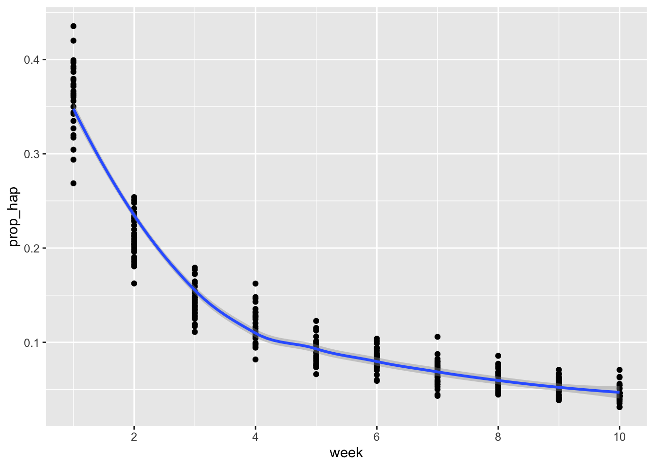
5.3 Normalizing sentiment
But as we discussed in the lecture, we also know that just because the total number of happy words increases, this isn’t indication on its own that we’re getting happier as a class over time.
Before we can begin to make any such inference, we need to normalize by the total number of words each week.
Below, I simulate data where the number of happy words is actually the same each week (our happyn dataset above).
I join these data with three other datasets: happylipsumn, happylipsumu, and happylipsumd. These are datasets of random text, with the same number of happy words.
The first of these also has the same number of total words each week. The second two, however, have differing number of total words each week: happylipsumu has an increasing number of total words each week; happylipsumd has a decreasing number of total words each week.
Again, as you see below, we’re splitting by week, student, word, and whether or not it is a “happy” word.
head(happylipsumn)## # A tibble: 6 × 4
## # Groups: week, student [1]
## week student word happy
## <int> <int> <chr> <int>
## 1 1 9 lorem 0
## 2 1 9 ipsum 0
## 3 1 9 dolor 0
## 4 1 9 sit 0
## 5 1 9 amet 0
## 6 1 9 semper 0
head(happylipsumu)## # A tibble: 6 × 4
## # Groups: week, student [1]
## week student word happy
## <int> <int> <chr> <int>
## 1 1 9 lorem 0
## 2 1 9 ipsum 0
## 3 1 9 dolor 0
## 4 1 9 sit 0
## 5 1 9 amet 0
## 6 1 9 commodo 0
head(happylipsumd)## # A tibble: 6 × 4
## # Groups: week, student [1]
## week student word happy
## <int> <int> <chr> <int>
## 1 1 9 lorem 0
## 2 1 9 ipsum 0
## 3 1 9 dolor 0
## 4 1 9 sit 0
## 5 1 9 amet 0
## 6 1 9 et 0Then if we plot the number of happy words divided by the number of total words each week for each student in each of these datasets, we get the below.
To get this normalized sentiment score–or “happy” score–we need to create a variable (column) in our dataframe that is the sum of happy words divided by the total number of words in the dataframe.
We can do this in the following way.
happylipsumn %>%
    group_by(week, student) %>%
    mutate(index_total = n()) %>%
    filter(happy==1) %>%
    summarise(sum_hap = sum(happy),
              index_total = index_total,
              prop_hap = sum_hap/index_total) %>%
    distinct()
## Warning: Returning more (or less) than 1 row per `summarise()` group was
## deprecated in dplyr 1.1.0.
## ℹ Please use `reframe()` instead.
## ℹ When switching from `summarise()` to `reframe()`, remember
## that `reframe()` always returns an ungrouped data frame and
## adjust accordingly.
## Call `lifecycle::last_lifecycle_warnings()` to see where this
## warning was generated.## `summarise()` has grouped output by 'week', 'student'. You can
## override using the `.groups` argument.## # A tibble: 300 × 5
## # Groups: week, student [300]
## week student sum_hap index_total prop_hap
## <int> <int> <int> <int> <dbl>
## 1 1 1 894 3548 0.252
## 2 1 2 1164 5259 0.221
## 3 1 3 1014 4531 0.224
## 4 1 4 774 3654 0.212
## 5 1 5 980 4212 0.233
## 6 1 6 711 3579 0.199
## 7 1 7 1254 5025 0.250
## 8 1 8 1117 4846 0.230
## 9 1 9 1079 4726 0.228
## 10 1 10 1061 5111 0.208
## # ℹ 290 more rowsThen if we repeat this for each of our datasets and plot we see the following.
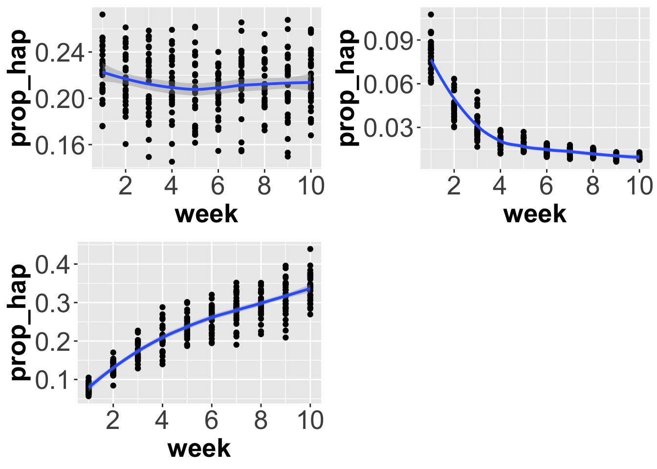
Why do the plots look like this?
Well, in the first, we have about the same number of total words each week and about the same number of happy words each week. If we divided the latter by the former, we get a proportion that is also stable over time.
In the second, however, we have an increasing number of total words each week, but about the same number of happy words over time. This means that we are dividing by an ever larger number, giving ever smaller proportions. As such, the trend is decreasing over time.
In the third, we have a decreasing number of total words each week, but about the same number of happy words over time. This means that we are dividing by an ever smaller number, giving ever larger proportions. As such, the trend is increasing over time.