3 Week 2 Demo

3.1 Setup

In this section, we’ll have a quick overview of how we’re processing text data when conducting analyses of word frequency. We’ll be using some randomly simulated text.

First we load the packages that we’ll be using:

library(stringi) #to generate random text
library(dplyr) #tidyverse package for wrangling data
library(tidytext) #package for 'tidy' manipulation of text data
library(ggplot2) #package for visualizing data
library(scales) #additional package for formatting plot axes
library(kableExtra) #package for displaying data in html format (relevant for formatting this worksheet mainly)

3.2 Tokenizing

We’ll first get some random text to see what it looks like when we’re tokenizing text.

lipsum_text <- data.frame(text = stri_rand_lipsum(1, start_lipsum = TRUE))

head(lipsum_text$text)

## [1] "Lorem ipsum dolor sit amet, mauris dolor posuere sed sit dapibus sapien egestas semper aptent. Luctus, eu, pretium enim, sociosqu rhoncus quis aliquam. In in in auctor natoque venenatis tincidunt. At scelerisque neque porta ut mi a, congue quis curae. Facilisis, adipiscing mauris. Dis non interdum cum commodo, tempor sapien donec in luctus. Nascetur ullamcorper, dui non semper, arcu sed. Sed non pellentesque rutrum tempor, curabitur in. Taciti gravida ut interdum iaculis. Arcu consectetur dictum et erat vestibulum luctus ridiculus! Luctus metus ad ex bibendum, eget at maximus nisl quisque ante posuere aptent. Cubilia tellus sed aliquam, suspendisse arcu et dapibus aenean. Ultricies primis sit nulla condimentum, sed, phasellus viverra nullam, primis."

We can then tokenize with the unnest_tokens() function in tidytext.

tokens <- lipsum_text %>%
  unnest_tokens(word, text)

head(tokens)

##     word
## 1  lorem
## 2  ipsum
## 3  dolor
## 4    sit
## 5   amet
## 6 mauris

Now we’ll get some larger data, simulating 5000 observations (rows) of random Latin text strings.

## Varying total words example
lipsum_text <- data.frame(text = stri_rand_lipsum(5000, start_lipsum = TRUE))

We’ll then add another column and call this “weeks.” This will be our unit of analysis.

# make some weeks one to ten
lipsum_text$week <- as.integer(rep(seq.int(1:10), 5000/10))

Now we’ll simulate a trend where we see an increasing number of words as weeks go by. Don’t worry too much about this as the code is a little more complex, but I share it here in case of interest.

for(i in 1:nrow(lipsum_text)) {
  week <- lipsum_text[i, 2]
  morewords <-
    paste(rep("more lipsum words", times = sample(1:100, 1) * week), collapse = " ")
  lipsum_words <- lipsum_text[i, 1]
  new_lipsum_text <- paste0(morewords, lipsum_words, collapse = " ")
  lipsum_text[i, 1] <- new_lipsum_text
}

And we can see that as each week goes by, we have more and more text.

lipsum_text %>%
  unnest_tokens(word, text) %>%
  group_by(week) %>%
  dplyr::count(word) %>%
  select(week, n) %>%
  distinct() %>%
  ggplot() +
  geom_bar(aes(week, n), stat = "identity") +
  labs(x = "Week", y = "n words") +
  scale_x_continuous(breaks= pretty_breaks())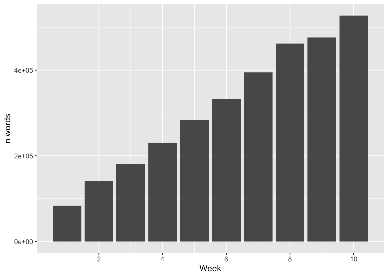

We can then do the same but with a trend where each week sees a decreasing number of words.

# simulate decreasing words trend
lipsum_text <- data.frame(text = stri_rand_lipsum(5000, start_lipsum = TRUE))

# make some weeks one to ten
lipsum_text$week <- as.integer(rep(seq.int(1:10), 5000/10))

for(i in 1:nrow(lipsum_text)) {
  week <- lipsum_text[i,2]
  morewords <- paste(rep("more lipsum words", times = sample(1:100, 1)* 1/week), collapse = " ")
  lipsum_words <- lipsum_text[i,1]
  new_lipsum_text <- paste0(morewords, lipsum_words, collapse = " ")
  lipsum_text[i,1] <- new_lipsum_text
}

lipsum_text %>%
  unnest_tokens(word, text) %>%
  group_by(week) %>%
  dplyr::count(word) %>%
  select(week, n) %>%
  distinct() %>%
  ggplot() +
  geom_bar(aes(week, n), stat = "identity") +
  labs(x = "Week", y = "n words") +
  scale_x_continuous(breaks= pretty_breaks())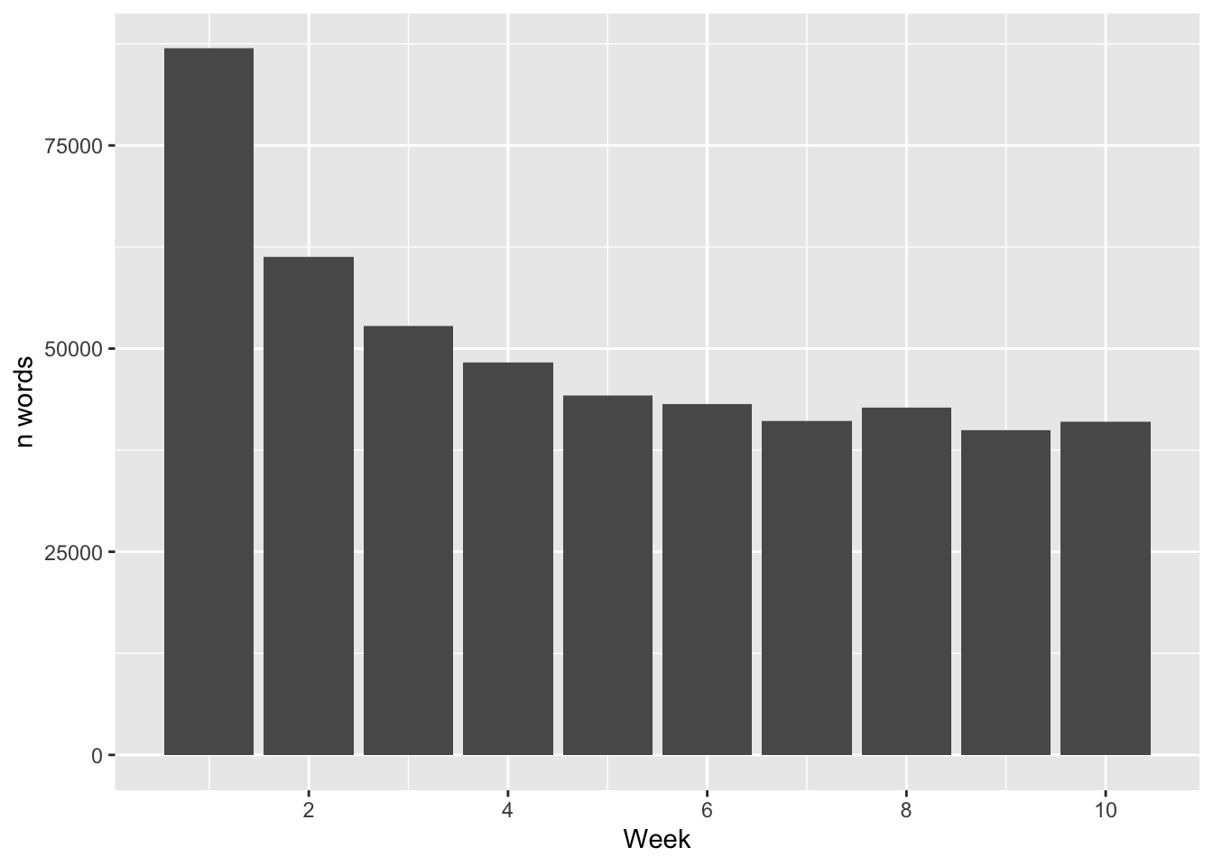

Now let’s check out the top frequency words in this text.

lipsum_text %>%
  unnest_tokens(word, text) %>%
  dplyr::count(word, sort = T) %>%
  top_n(5) %>%
  knitr::kable(format="html")%>% 
  kable_styling("striped", full_width = F)

## Selecting by n

word	n
lipsum	72170
more	72170
words	67407
sed	17608
in	12437

We’re going to check out the frequencies for the word “sed” and then we’re gonna normalize these by denominating by total word frequencies for each week.

First we need to get total word frequencies for each week.

lipsum_totals <- lipsum_text %>%
  group_by(week) %>%
  unnest_tokens(word, text) %>%
  dplyr::count(word) %>%
  mutate(total = sum(n)) %>%
  distinct(week, total)

# let's look for "sed"
lipsum_sed <- lipsum_text %>%
  group_by(week) %>%
  unnest_tokens(word, text) %>%
  filter(word == "sed")  %>%
  dplyr::count(word) %>%
  mutate(total_sed = sum(n)) %>%
  distinct(week, total_sed)

Then we can join these two dataframes together with the left_join() function where we’re joining by the “week” column. We can then pipe the joined data into a plot.

lipsum_sed %>%
  left_join(lipsum_totals, by = "week") %>%
  mutate(sed_prop = total_sed/total) %>%
  ggplot() +
  geom_line(aes(week, sed_prop)) +
  labs(x = "Week", y = "
       Proportion sed word") +
  scale_x_continuous(breaks= pretty_breaks())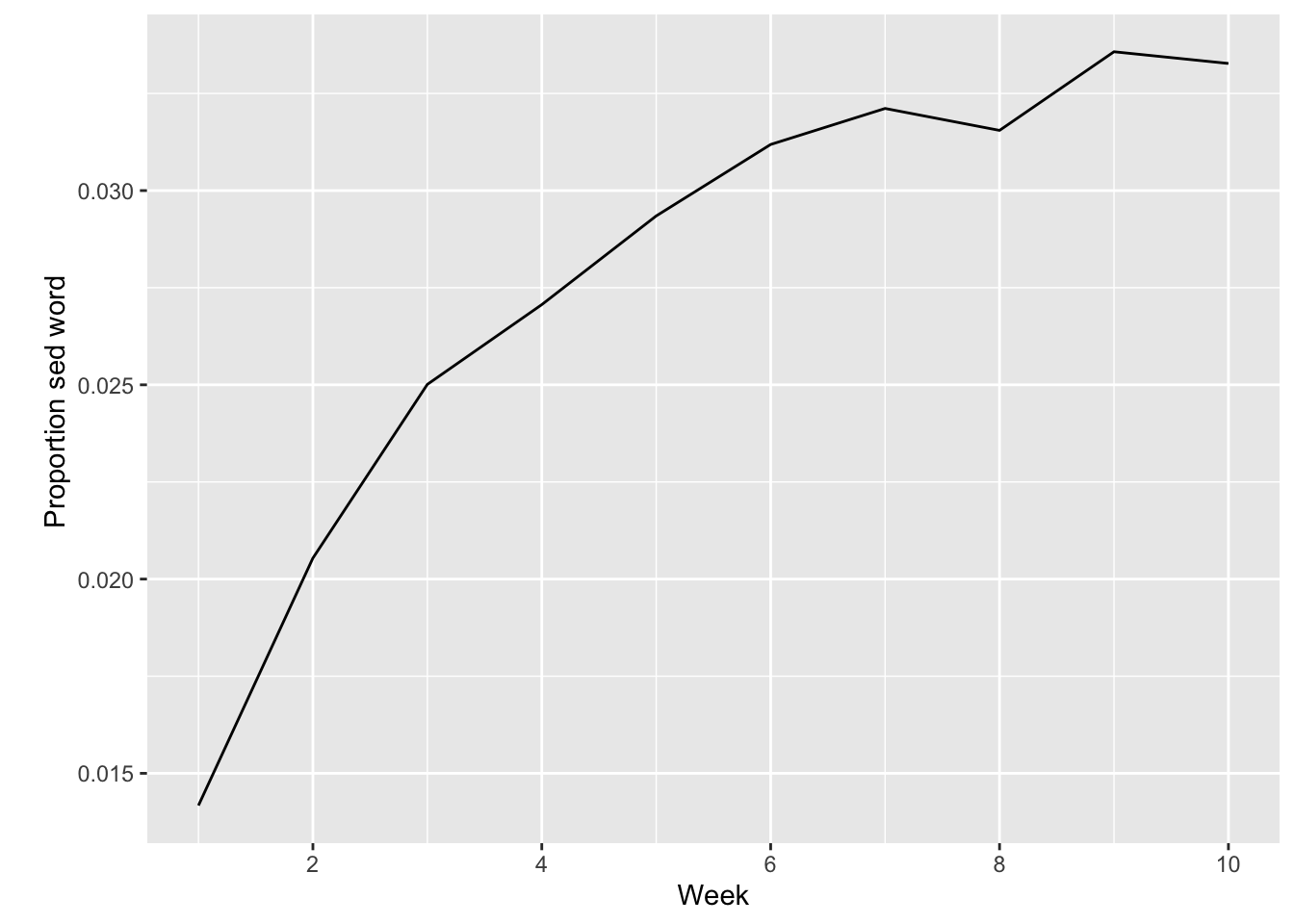

3.3 Regexing

You’ll notice that in the worksheet on word frequencies that at one point there are a set of parentheses after str_detect() we have the string “[a-z]”. This is called a character class and these use square brackets like [].

Other character classes include, as helpfully listed in this vignette for the stringr package. What follows is adapted from these materials on regular expressions.

[abc]: matches a, b, or c.
[a-z]: matches every character between a and z (in Unicode code point order).
[^abc]: matches anything except a, b, or c.
[\^\-]: matches ^ or -.

Several other patterns match multiple characters. These include:

\d: matches any digit; the opposite of this is \D, which matches any character that is not a decimal digit.

str_extract_all("1 + 2 = 3", "\\d+")

## [[1]]
## [1] "1" "2" "3"

str_extract_all("1 + 2 = 3", "\\D+")

## [[1]]
## [1] " + " " = "

\s: matches any whitespace; its opposite is \S

(text <- "Some  \t badly\n\t\tspaced \f text")

## [1] "Some  \t badly\n\t\tspaced \f text"

str_replace_all(text, "\\s+", " ")

## [1] "Some badly spaced text"

^: matches start of the string

x <- c("apple", "banana", "pear")
str_extract(x, "^a")

## [1] "a" NA  NA

$: matches end of the string

x <- c("apple", "banana", "pear")
str_extract(x, "^a$")

## [1] NA NA NA

^ then $: exact string match

x <- c("apple", "banana", "pear")
str_extract(x, "^apple$")

## [1] "apple" NA      NA

Hold up: what do the plus signs etc. mean?

+: 1 or more.
*: 0 or more.
?: 0 or 1.

So if you can tell me why this output makes sense, you’re getting there!

str_extract_all("1 + 2 = 3", "\\d+")[[1]]

## [1] "1" "2" "3"

str_extract_all("1 + 2 = 3", "\\D+")[[1]]

## [1] " + " " = "

str_extract_all("1 + 2 = 3", "\\d*")[[1]]

##  [1] "1" ""  ""  ""  "2" ""  ""  ""  "3" ""

str_extract_all("1 + 2 = 3", "\\D*")[[1]]

## [1] ""    " + " ""    " = " ""    ""

str_extract_all("1 + 2 = 3", "\\d?")[[1]]

##  [1] "1" ""  ""  ""  "2" ""  ""  ""  "3" ""

str_extract_all("1 + 2 = 3", "\\D?")[[1]]

##  [1] ""  " " "+" " " ""  " " "=" " " ""  ""

3.3.1 Some more regex resources:

Regex crossword: https://regexcrossword.com/.
Regexone: https://regexone.com/
R4DS chapter 14

2 Week 2: Tokenization and word frequencies

4 Week 3: Dictionary-based techniques