20 Exercise 4: Scaling techniques
20.1 Introduction
The hands-on exercise for this week focuses on: 1) scaling texts ; 2) implementing scaling techniques using quanteda.
In this tutorial, you will learn how to:
- Scale texts using the “wordfish” algorithm
- Scale texts gathered from online sources
- Replicate analyses by Kaneko, Asano, and Miwa (2021)
Before proceeding, we’ll load the packages we will need for this tutorial.
library(dplyr)
library(quanteda) # includes functions to implement Lexicoder
library(quanteda.textmodels) # for estimating similarity and complexity measures
library(quanteda.textplots) #for visualizing text modelling results
In this exercise we’ll be using the dataset we used for the sentiment analysis exercise. The data were collected from the Twitter accounts of the top eight newspapers in the UK by circulation. The tweets include any tweets by the news outlet from their main account.
20.2 Importing data
We can download the dataset with:
tweets <- readRDS("data/sentanalysis/newstweets.rds")If you’re working on this document from your own computer (“locally”) you can download the tweets data in the following way:
tweets <- readRDS(gzcon(url("https://github.com/cjbarrie/CTA-ED/blob/main/data/sentanalysis/newstweets.rds?raw=true")))We first take a sample from these data to speed up the runtime of some of the analyses.
20.3 Construct dfm object
Then, as in the previous exercise, we create a corpus object, specify the document-level variables by which we want to group, and generate our document feature matrix.
#make corpus object, specifying tweet as text field
tweets_corpus <- corpus(tweets, text_field = "text")

#add in username document-level information
docvars(tweets_corpus, "newspaper") <- tweets$user_username

dfm_tweets <- dfm(tokens(tweets_corpus),
                  remove_punct = TRUE,
                  remove = stopwords("english"))
We can then have a look at the number of documents (tweets) we have per newspaper Twitter account.
##
##     DailyMailUK     DailyMirror EveningStandard        guardian
##            2052            5834            2182            2939
##         MetroUK       Telegraph          TheSun        thetimes
##             966            1519            3840             668
And this is what our document feature matrix looks like, where each word has a count for each of our eight newspapers.
dfm_tweets## Document-feature matrix of: 20,000 documents, 48,967 features (99.98% sparse) and 31 docvars.
## features
## docs rt @standardnews breaking coronavirus outbreak declared
## text1 1 1 1 1 1 1
## text2 1 0 0 0 0 0
## text3 0 0 0 0 0 0
## text4 0 0 0 0 0 0
## text5 0 0 0 0 0 0
## text6 0 0 0 0 0 0
## features
## docs pandemic world health organisation
## text1 1 1 1 1
## text2 0 0 0 0
## text3 0 0 0 0
## text4 0 0 0 0
## text5 0 0 0 0
## text6 0 0 0 0
## [ reached max_ndoc ... 19,994 more documents, reached max_nfeat ... 48,957 more features ]20.4 Estimate wordfish model
Once we have our data in this format, we are able to group and trim the document feature matrix before estimating the wordfish model.
# compress the document-feature matrix at the newspaper level
dfm_newstweets <- dfm_group(dfm_tweets, groups = newspaper)
# remove words not used by two or more newspapers
dfm_newstweets <- dfm_trim(dfm_newstweets,
                                min_docfreq = 2, docfreq_type = "count")

## size of the document-feature matrix
dim(dfm_newstweets)
## [1] 8 11111
#### estimate the Wordfish model ####
set.seed(123L)
dfm_newstweets_results <- textmodel_wordfish(dfm_newstweets,
                                             sparse = TRUE)
And this is what results.
summary(dfm_newstweets_results)##
## Call:
## textmodel_wordfish.dfm(x = dfm_newstweets, sparse = TRUE)
##
## Estimated Document Positions:
## theta se
## DailyMailUK 0.64904 0.012949
## DailyMirror 1.18235 0.006726
## EveningStandard -0.22616 0.016082
## guardian -0.95429 0.010563
## MetroUK -0.04625 0.022759
## Telegraph -1.05344 0.010640
## TheSun 1.45044 0.006048
## thetimes -1.00168 0.014966
##
## Estimated Feature Scores:
## rt breaking coronavirus outbreak declared pandemic
## beta 0.537 0.191 0.06918 -0.2654 -0.06526 -0.2004
## psi 5.307 3.535 5.78715 3.1348 0.50705 3.1738
## world health organisation genuinely interested see
## beta -0.317 -0.3277 -0.4118 -0.2873 -0.2545 0.0005106
## psi 3.366 3.2041 0.5487 -0.5403 -1.4502 2.7723965
## one cos fair german care system protect
## beta -0.06313 -0.2788 -0.03078 -0.7424 -0.3251 -1.105 -0.1106
## psi 3.85881 -1.4480 0.35480 1.1009 3.1042 1.259 1.8918
## troubled children #covid19 anxiety shows sign man
## beta -0.4731 0.01205 -0.6742 0.4218 0.4165 -0.1215 0.5112
## psi -0.0784 2.85004 2.9703 0.5917 2.8370 1.9427 3.5777
## behind app explains tips
## beta 0.05499 0.271 0.6687 -0.2083
## psi 2.43805 1.376 1.2749 1.5341We can then plot our estimates of the \(\theta\)s—i.e., the estimates of the latent newspaper position—as so.
textplot_scale1d(dfm_newstweets_results)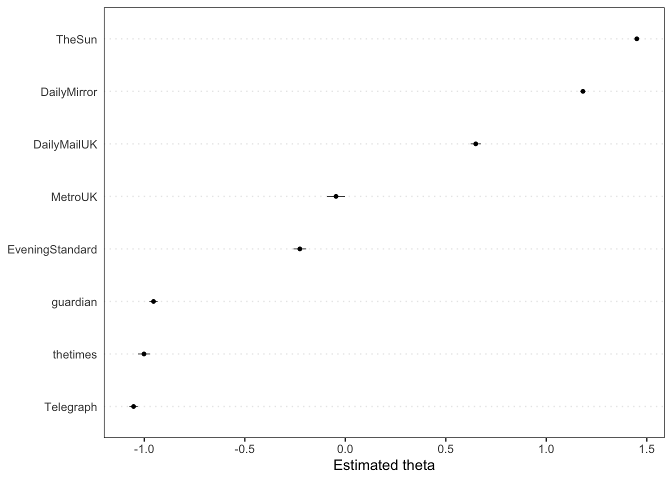
Interestingly, we seem not to have captured ideology but some other tonal dimension. We see that the tabloid newspapers are scored similarly, and grouped toward the right hand side of this latent dimension; whereas the broadsheet newspapers have an estimated theta further to the left.
Plotting the “features,” i.e., the word-level betas shows how words are positioned along this dimension, and which words help discriminate between news outlets.
textplot_scale1d(dfm_newstweets_results, margin = "features")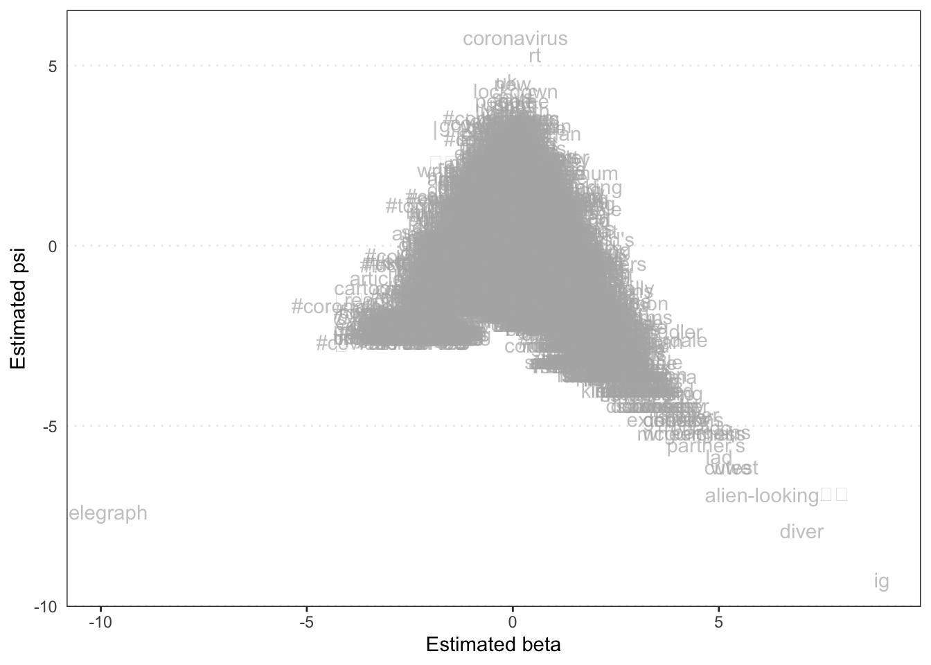
And we can also look at these features.
features <- dfm_newstweets_results[["features"]]

betas <- dfm_newstweets_results[["beta"]]

feat_betas <- as.data.frame(cbind(features, betas))
feat_betas$betas <- as.numeric(feat_betas$betas)

feat_betas %>%
  arrange(desc(betas)) %>%
  top_n(20) %>%
  kbl() %>%
  kable_styling(bootstrap_options = "striped")
## Selecting by betas| features | betas |
|---|---|
| ig | 8.961658 |
| 🎥 | 7.789175 |
| diver | 7.015284 |
| alien-looking | 6.054602 |
| wwe | 5.304745 |
| cutest | 5.304745 |
| lad | 5.012236 |
| bargains | 4.835000 |
| partner’s | 4.692455 |
| ronaldo | 4.495503 |
| clever | 4.351121 |
| wheelchair | 4.340554 |
| mcguinness | 4.340554 |
| spider | 4.192177 |
| nails | 4.192177 |
| rides | 3.950629 |
| ghostly | 3.950629 |
| extensions | 3.950629 |
| corrie’s | 3.950629 |
| lion | 3.857076 |
These words do seem to belong to more tabloid-style reportage, and include emojis relating to film, sports reporting on “cristiano” as well as more colloquial terms like “saucy.”
20.5 Replicating Kaneko et al.
This section adapts code from the replication data provided for Kaneko, Asano, and Miwa (2021) here. We can access data from the first study by Kaneko, Asano, and Miwa (2021) in the following way.
kaneko_dfm <- readRDS("data/wordscaling/study1_kaneko.rds")If you’re working locally, you can download the dfm data with:
kaneko_dfm <- readRDS(gzcon(url("https://github.com/cjbarrie/CTA-ED/blob/main/data/wordscaling/study1_kaneko.rds?raw=true")))This data is in the form a document-feature-matrix. We can first manipulate it in the same way as Kaneko, Asano, and Miwa (2021) by grouping at the level of newspaper and removing infrequent words.
##
##       Asahi     Chugoku    Chunichi    Hokkaido      Kahoku
##          38          24          47          46          18
##    Mainichi      Nikkei Nishinippon      Sankei     Yomiuri
##          26          13          27          14          30
## prepare the newspaper-level document-feature matrix
# compress the document-feature matrix at the newspaper level
kaneko_dfm_study1 <- dfm_group(kaneko_dfm, groups = Newspaper)
# remove words not used by two or more newspapers
kaneko_dfm_study1 <- dfm_trim(kaneko_dfm_study1, min_docfreq = 2, docfreq_type = "count")

## size of the document-feature matrix
dim(kaneko_dfm_study1)
## [1] 10 466020.6 Exercises
- Estimate a wordfish model for the Kaneko, Asano, and Miwa (2021) data
- Visualize the results