11 Week 6 Demo
11.1 Setup
First, we’ll load the packages we’ll be using in this week’s brief demo.
Estimating a topic model requires us first to have our data in the form of a document-term-matrix. This is another term for what we have referred to in previous weeks as a document-feature-matrix.
We can take some example data from the topicmodels package. This text is from news releases by the Associated Press. It consists of around 2,200 articles (documents) and over 10,000 terms (words).
data("AssociatedPress",
     package = "topicmodels")
To estimate the topic model we need only to specify the document-term-matrix we are using, and the number (k) of topics that we are estimating. To speed up estimation, we are here only estimating it on 100 articles.
lda_output <- LDA(AssociatedPress[1:100,], k = 10)We can then inspect the contents of each topic as follows.
terms(lda_output, 10)## Topic 1 Topic 2 Topic 3 Topic 4
## [1,] "percent" "police" "soviet" "central"
## [2,] "new" "i" "union" "noriega"
## [3,] "company" "man" "year" "peres"
## [4,] "oil" "state" "president" "official"
## [5,] "duracell" "fire" "questions" "panama"
## [6,] "gas" "new" "bar" "snow"
## [7,] "million" "rating" "batalla" "nation"
## [8,] "year" "three" "last" "northern"
## [9,] "record" "greyhound" "multistate" "president"
## [10,] "prices" "mrs" "officials" "southern"
## Topic 5 Topic 6 Topic 7 Topic 8 Topic 9
## [1,] "two" "i" "percent" "soviet" "bush"
## [2,] "year" "bush" "year" "new" "dukakis"
## [3,] "roberts" "barry" "prices" "officers" "i"
## [4,] "soviet" "campaign" "month" "polish" "people"
## [5,] "years" "moore" "rate" "florio" "waste"
## [6,] "people" "study" "report" "settlements" "warming"
## [7,] "congress" "like" "months" "union" "global"
## [8,] "i" "asked" "economy" "exxon" "city"
## [9,] "north" "children" "rose" "government" "front"
## [10,] "officials" "last" "index" "money" "president"
## Topic 10
## [1,] "new"
## [2,] "bank"
## [3,] "administration"
## [4,] "california"
## [5,] "percent"
## [6,] "farmer"
## [7,] "i"
## [8,] "thats"
## [9,] "magellan"
## [10,] "spacecraft"We can then use the tidy() function from tidytext to gather the relevant parameters we’ve estimated. To get the \(\beta\) per-topic-per-word probabilities (i.e., the probability that the given term belongs to a given topic) we can do the following.
## # A tibble: 104,730 × 3
##    topic term      beta
##    <int> <chr>    <dbl>
##  1     7 percent 0.0331
##  2    10 new     0.0165
##  3    10 bank    0.0159
##  4     8 soviet  0.0150
##  5     1 percent 0.0122
##  6     9 bush    0.0118
##  7     9 dukakis 0.0118
##  8     8 new     0.0111
##  9     2 police  0.0104
## 10     6 i       0.0103
## # ℹ 104,720 more rows
And to get the \(\gamma\) per-document-per-topic probabilities (i.e., the probability that a given document (here: article) belongs to a particular topic) we do the following.
## # A tibble: 1,000 × 3
##    document topic gamma
##       <int> <int> <dbl>
##  1       76    10  1.00
##  2       81     4  1.00
##  3        6     4  1.00
##  4       43     5  1.00
##  5       95    10  1.00
##  6       77     9  1.00
##  7       29     8  1.00
##  8       80     1  1.00
##  9       57     5  1.00
## 10       25    10  1.00
## # ℹ 990 more rows
And we can easily plot our \(\beta\) estimates as follows.
lda_beta %>%
  group_by(topic) %>%
  top_n(10, beta) %>%
  ungroup() %>%
  arrange(topic, -beta) %>%
  mutate(term = reorder_within(term, beta, topic)) %>%
  ggplot(aes(beta, term, fill = factor(topic))) +
  geom_col(show.legend = FALSE) +
  facet_wrap(~ topic, scales = "free", ncol = 4) +
  scale_y_reordered() +
  theme_tufte(base_family = "Helvetica")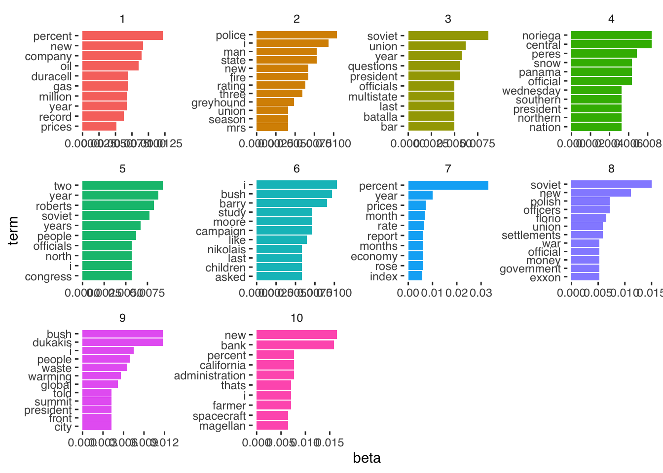
Which shows us the words associated with each topic, and the size of the associated \(\beta\) coefficient.